An intuitive explanation and use cases of PCA

Principal component analysis (PCA) is a very popular technique used for dimensionality reduction. It is an unsupervised learning technique used for transforming data. It is unsupervised since it does not consider the target predictor into consideration while analyzing and transforming the data. The outcome of PCA are new transformed predictors which are orthogonal to each other and summarize the variance of input predictors.

The objective of this article is to give an intuitive explanation of what PCA does with help of analogies and to provide with various scenarios where this algorithm can come handy. We are not going to go in depth about the mathematics of PCA, rather we will present the core idea behind the algorithm.

By the end of this article, you will understand:

• The core idea behind PCA
• Why having too many predictors can be problematic
• How PCA solves the problem of curse of dimensionality
• Other applications of PCA
• Implementation of PCA using scikit-learn package in Python

Curse of dimensionality: No more features please

Usually we will be more than happy to have huge volume of data to solve our predictive modeling problem. We believe that more data often leads to better results. By more data, data which has high volume vise and many predictors. This is in fact true for some of the problems. Then why doesn’t it work in every case. The answer is simple, there is some similarity between the dimensions or features or predictors. And not just that, some of them are pretty much have zero contribution to our target variable. This will increase the complication and runtime of our model while having no effect on accuracy. This can be termed as curse of dimensionality, which simply is that useless or co-related predictors over-fitting or increasing the complexity of our model.

This is an usual scenario when dealing with image data and few other situations. Not all the features have equal contribution to target variable. Correlated predictors tend to over-contribute to the model leading to high variance. It is crucial to transform the such that correlated features are merged to minimize the variance of our model. PCA can help us achieve the same by rotating the axes along the direction of maximum variance of our existing features. This may sound complex but trust me, this will become easy as we go through it more deeply.

PCA: A basic intuition

intuition

A predictor with maximum variance is likely to have maximum impact on target variable

Let us start our understanding of PCA with the help of an example problem containing two features, $x_1$, $x_2$ and a target variable y. Later we shall have generalized theory that holds good for more complex data. Let us also assume that $x_1$ and $x_2$ are correlated and are plotted in $Fig 1$. There is clearly a linear relationship between the predictors and is shown by the $red line$.

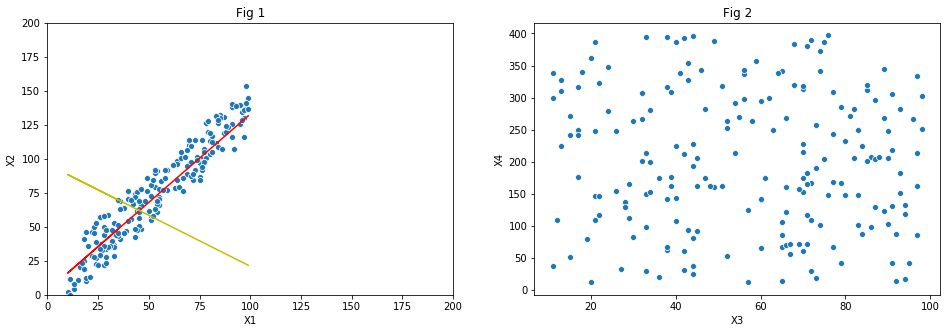
As you can see in the plot, majority of points are either on the line or lying close it and are spread across the length of it. We can rephrase the above statement as ’$x_1$ and $x_2$ have maximum variance along the red line’. Next highest variance is along the line perpendicular to the linear fit. Roughly 90% of variance is along the red line and rest along the yellow line. Note here that we are talking about the direction of variance and not the points lying on the mentioned lines.

This is exactly what PCA utilizes. It will rotate our axes along the direction of highest variance. The next highest variance can be observed along the direction perpendicular to the previous direction. In case of two dimensional problems we get new two directions which are perpendicular to each other along the directions of maximum variance. For a multidimensional problem having n predictors we get n principal components in descending order. That is, first principal component will have the maximum variance followed second and so on. Also all of the principal components are orthogonal to each other.

$$X_1,X_2,X_3,....,X_n = PCA(x_1,x_2,x_3,...,x_n)$$ $$X_i = \beta_0 + \sum_{i=0}^n \beta_ix_i$$

From the above equations it can be clearly seen that each principal component is a linear combination of all the predictors. $\beta_i$ represents the weight for the predictor $x_i$, which indicates the strength of variance of $x_i$ on that particular principal component. In total we get $n$ principal components for $n$ predictors, although it is up to us to keep them all or discard few components based on some criteria.

Properties of principal components:

1. Unsupervised transformation technique
2. Principal components are orthogonal. So there is no correlation among them
3. They align in the direction of maximum variance (in descending order)

But why variance?

The whole concept of PCA runs on an assumption that variance in data is the key indicator of strength of a predictor. It believes that predictor with high variance has the greatest impact on the target variable while keeping other predictors into consideration. That means we are not independently evaluating the variance of a predictor, we are in fact throwing all the points in $n$ dimensional space and measuring the variance.

How does PCA solve the problem of ‘Curse of dimensionality’?

When we compute the principal components of our original $n$ dimensions, we get $n$ new orthogonal components. Each one of the components carry some information about variance. For example, first one might have $32$% of variance, second one might carry $21$% etc. We can set a threshold value of variance, $p$, and set a condition saying first $k$ components whose variance sum up to $p$ can be kept (say $k$) and rest $n-k$ can be discarded. For a well selected value (usual value is $95$%), we can safely say that majority of information is retained as the discarded components carry little variance anyway.

This is especially helpful if the number of starting dimensions, $n$, is very large (in the order 1000). By wisely selecting the threshold, we can reduce the number of dimensions to the order of 100. This will give a significant boost to computation, improves the model interpretability and helps in overcoming the variance issue due to high dimensions of untransformed data.

Principal components vs Collinearity

Collinearity is the situation where independent variables are highly correlated. The relation between the those correlated variables can be linear or non-linear. This results in inflation regression coefficient (weight) for those variables resulting in an undependable model that performs poorly. It is in fact highly recommended to get rid of correlated predictors even before we start building our predictive model. During data transformation we need create new feature out of these redundant features or if necessary get rid of them entirely.

PCA can come handy to study the collinearity of predictors. Remember that the core idea behind PCA is to study the variance of predictors in a multi-dimensional state and build new dimensions which are orthogonal along the direction of highest variance. When two or more predictors are correlated, like in $Fig 1$ they tend spread only along one direction. On the other hand uncorrelated features tend to spread across the space as shown in $Fig 2$.

Therefore the few principal components of correlated predictors carry maximum information about the variance and thus can replace the original features for the purpose of predictive modeling. The variance distribution among principal components for the example shown in Fig 1 are 90% and 10% for components 1 and 2 respectively. So by just having component $X_1$, we can retain 90% of variance, and thus 90% of information carried by $x_1$ and $x_2$. Thus two components are now reduced to one while retaining majority of information. In case of Fig 2, first two principal components have 55% and 45% of variance and are just as good as original predictors. So we will not gain anything by resolving the original predictors into their principal components.

By retaining these principal components which carry maximum information (variance), we can eliminate redundant features without loss of information. This will result in better performance since the number of dimensions after PCA are lower than they were before and also we are eliminating collinear features resulting in a robust model that can well generalize the data. Although PCA can help us deal with collinearity care must be taken as it only considers the variance of the features and not their actual contribution towards the target variable. An irrelevant feature with maximum variance will have high contribution than an important feature with lower variance. This is one of the shortcomings of PCA and the reason behind it is that it is an unsupervised feature transformation technique. More of the drawbacks of PCA are listed below.

Drawbacks of PCA

• Doesn’t take into consideration the relationship between a predictor and the target variable, aka, unsupervised technique
• Assumes that variance is the only indicator to determine the importance of a feature. No other statistical estimates are considered for feature transformation
• Features with similar variance does not benefit through PCA
• Principal components are computed using several complex algorithms which are not straightforward. (SVD is most popular among them)

Implementation using Sklearn

Python’s sklearn has multiple matrix decomposition techniques clubbed under single module called decomposition. There are multiple variations of PCA like regular PCA, Kernel PCA, Sparse PCA, Incremental PCA and Mini batch sparse PCA. We shall discuss the implementation standard PCA which is the most used one. Other variants also follow the same structure when it comes to implementation using sklearn.

#import module
from sklearn.decomposition import PCA

#create PCA object
pca = PCA(n_components=2)

#fit PCA object to our data. Outputs the principle components in ascending order of variance
x_componants = pca.fit_transform(X)

#prints the variance ratio in increasing order
print(pca.explained_variance_ratio_)